Batch effects, technical variation and other sources of unwanted or spurious variation are ever-present in big data, especially so in high-throughput molecular (gene expression, proteomic or methylation) profiling. Fortunately, multiple methods exist for removing such variation that are suitable for various situations one may encounter. When a source of unwanted variation is known and can be represented by a numeric or categorical variable (such as batch), the variation can be adjusted for using regression models. The best-known method for molecular data, ComBat, works for categorical confounders only; primarily because of this limitation, I implemented a similar, empirical Bayes moderated linear model adjustment in function empiricalBayesLM in WGCNA. This function works for both categorical and continuous confounders, but only adjusts the mean, while ComBat also adjusts variation.
Whether working with categorical or numeric confounders, it is sometimes desirable to adjust the data such that only a subset of samples are used for the mean and possibly variance equalization. As an example, one may wish to merge two data sets, generated by different authors, in different labs and at different times, each containing control and disease samples, with a different disease in each set. Since molecular profiles of the two diseases may be different, it does not make sense to include these samples in the mean and variance adjustment; the adjustment coefficients (shifts and scalings) should be based only on the control samples but should be applied to all samples. For simplicity, assume that the only (strong) source of technical variation is the batch effect between the two sets.
In the WGCNA function empiricalBayesLM, the user can use the argument fitToSamples to specify which samples should be used in determining the adjustment coefficients; in the example of two sets, one would supply the indices of the control samples from both sets. The disease samples do not enter the calculation of coefficients but are then adjusted together with the control samples.
Although ComBat does not let the user specify a subset of samples to which the models should be fit, one can use the argument ‘mod’ (the model matrix of outcome of interest and other covariates) to achieve substantially the same effect. One could also use this approach with empiricalBayesLM, but there is a price to pay: including the disease variables in the model means their effect is first regressed out (together with the batch effect), then added back to the data (without the batch effect, of course). This can sometimes introduce artifacts and inflate significance in downstream analyses, as pointed out in a 2016 article by Nygaard and collaborators.
I will illustrate the two different approaches on simulated data. I will use a very simple simulation with normally distributed variables; the aim is to illustrate the batch correction, not to simulate realistic (say gene expression) data. The first chunk of code sets up the R session and simulates the two “data sets”. Copy and paste the code below into an R session (make sure you have packages sva and WGCNA installed) to try it yourself.
library(sva)
library(WGCNA)
options(stringsAsFactors = FALSE);

nGenes = 1000;
nSamples1 = 8;
nSamples2 = 12;
disEffect = 0.5;
batchEffect = 0.4;
set.seed(2);
# Simulate first data set, genes in columns
data1 = matrix(rnorm(nSamples1 * nGenes), nSamples1, nGenes)
annotation1 = data.frame(
      status = sample(c("Ctrl", "Disease1"), nSamples1, replace = TRUE));
# Add a global effect of disaese
dSamples1 = annotation1$status=="Disease1"
data1[ dSamples1, ] = data1[ dSamples1, ] +
      disEffect * matrix(rnorm(nGenes), sum(dSamples1), nGenes, byrow = TRUE)
# Simulate second data set
data2 = matrix(rnorm(nSamples2 * nGenes), nSamples2, nGenes)
annotation2 = data.frame(
     status = sample(c("Ctrl", "Disease2"), nSamples2, replace = TRUE));
# Add a global effect of disaese
dSamples2 = annotation2$status=="Disease2";
data2[ dSamples2, ] = data2[ dSamples2, ] +
      disEffect * matrix(rnorm(nGenes), sum(dSamples2), nGenes, byrow = TRUE)

# Add a batch effect to second data set: shift each gene by a random amount
data2 = data2 + batchEffect * matrix(rnorm(nGenes), nSamples2, nGenes, byrow = TRUE)

# Prepare a function to plot principal components since we will use it a few times
plotPCA = function(data, annotation, ...)
{
  svd1 = svd(data, nu = 2, nv = 0);
  status = annotation$status;
  ctrlSamples = status=="Ctrl"
  status[ctrlSamples] = paste0(status[ctrlSamples], annotation$batch[ctrlSamples])
  layout(matrix(c(1:2), 1, 2), widths = c(0.3, 1))
  par(mar = c(3.2, 0, 0, 0));
  plot(c(0, 1), type = "n", axes = FALSE,
       xlab = "", ylab = "");
  legend("bottomright", legend = sort(unique(status)),
         pch = 20 + c(1:length(unique(status))),
         pt.bg = labels2colors(1:length(unique(status))),
         pt.cex = 2)
  par(mar = c(3.2, 3.2, 2, 1))
  par(mgp = c(2, 0.7, 0))
  plot(svd1$u[, 1], svd1$u[, 2],
       xlab = "PC1", ylab = "PC2",
       pch = 20 + as.numeric(factor(status)),
       cex = 2.5, bg = labels2colors(status), cex.main = 1.0, ...)

}
The next chunk is where the common analysis starts. The two sets are merged and I plot the first two principal components of the merged data.
# Merge the two data sets
data = rbind(data1, data2)
# Include a batch variable in the combined sample annotation
annotation = data.frame(
    rbind(annotation1, annotation2),
    batch = c(rep(1, nSamples1), rep(2, nSamples2)))
# Plot PCs of the merged data
plotPCA(data, annotation,
    main = "Merged data before batch correction"

The samples separate cleanly into 4 groups; the difference between the two control groups is the batch effect.
# Correct for the batch effect using empiricalBayesLM from WGCNA
data.eblm = empiricalBayesLM(
   data,
   removedCovariates = annotation$batch,
   fitToSamples = annotation$status=="Ctrl")$adjustedData;
# See how well the correction worked
plotPCA(data.eblm, annotation,
        main = "Corrected by regression on control samples")
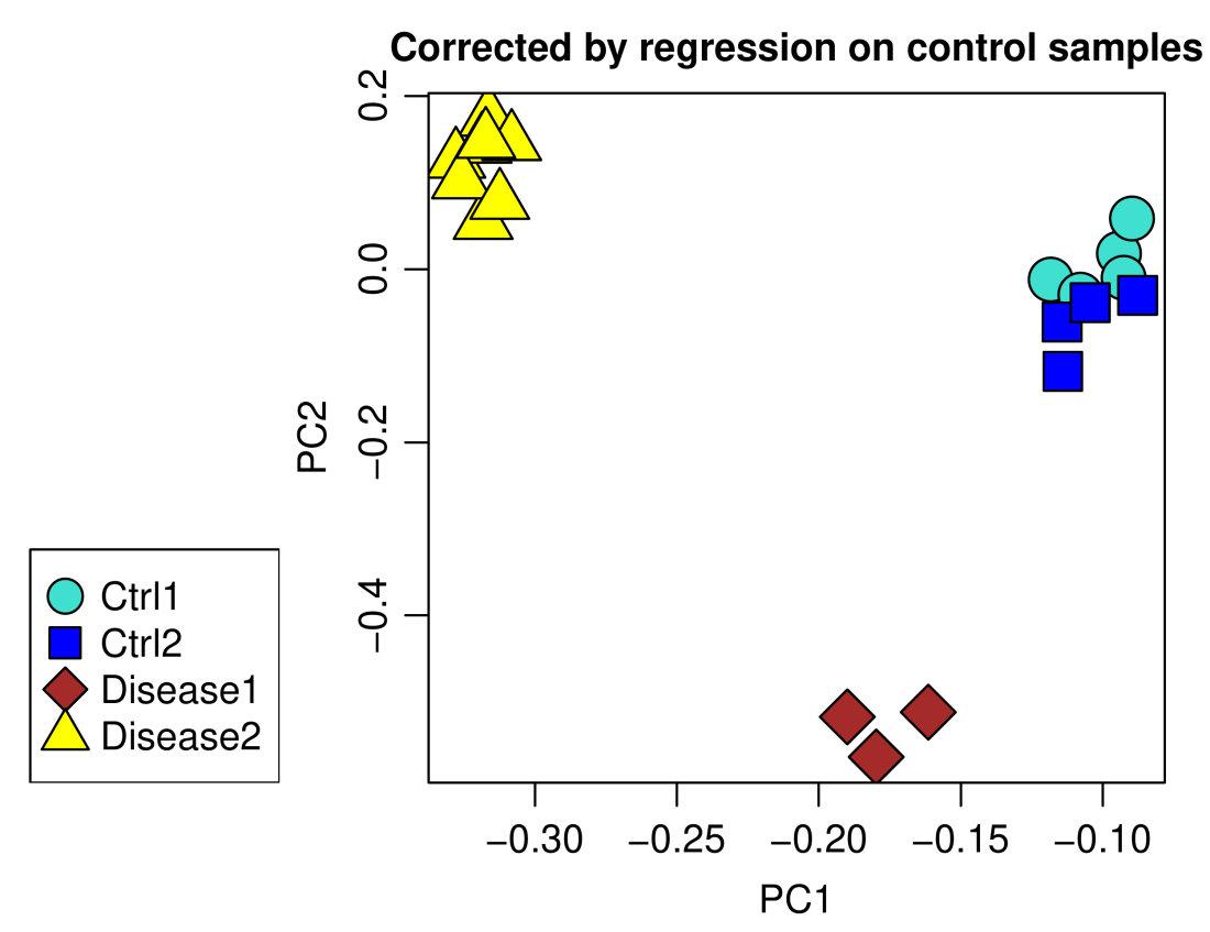
A residual batch effect is still apparent and can be removed using ordinary linear regression rather than empirical Bayes-moderated one, at the expense of possibly introducing some over-fitting. Since empiricalBayesLM also returns data corrected using plain linear models, the code is very similar. The component adjustedData of the output of empiricalBayesLM is simply replaced by adjustedData.OLS, OLS standing for ordinary least squares:
data.lm = empiricalBayesLM(data, removedCovariates = annotation$batch,
   fitToSamples = annotation$status=="Ctrl")$adjustedData.OLS;
# See how well the correction worked
plotPCA(data.lm, annotation,
        main = "Unmoderated regression on control samples")
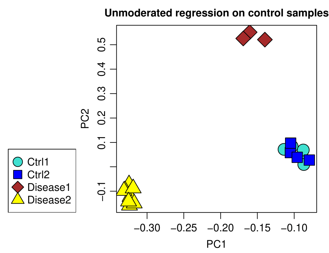
Using plain linear models indeed removed the batch effect completely.
It’s ComBat‘s turn now. I first show how a naive application of ComBat to correct the batch effect, without regard for disease status, leads to incorrect batch correction.
data.ComBat.naive = t(ComBat(t(data), batch = annotation$batch))
plotPCA(data.ComBat.naive, annotation,
        main = "Naive application of ComBat")
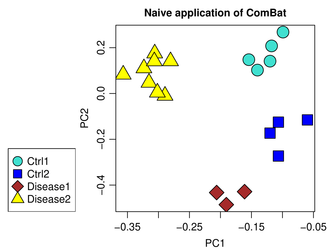
A major separation remains between the two groups of control samples, certainly not what one would like or expect from a successful batch correction. The correct approach is to include covariates of interest that encode the disease status in two separate indicator variables, one for each disease.
data.ComBat = t(ComBat(t(data), batch = annotation$batch,
                       mod = model.matrix(~status, data = annotation)))
plotPCA(data.ComBat, annotation,
        main = "Correct application of ComBat")
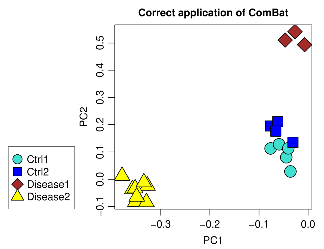
The result looks very much like the correction using empiricalBayesLM above, including the residual batch effect, but the results are not exactly the same – the approaches are in some ways equivalent but do not yield identical results. The upshot is that one can use both empiricalBayesLM and ComBat to achieve similar effect. The advantage of empiricalBayesLM is that it is more flexible: One can specify the samples to which the linear models should be fit rather than have to include extra covariates of interest. Since empiricalBayesLM avoids the two-step “regress out-add back in” procedure and its potential instabilities, one can also use plain linear model for adjustment to remove the batch effect completely. On the flip side, if the number of suitable samples is low (such as if there are only a few control and many disease samples), it may be better to include all samples and the additional covariates in the calculation, perhaps introducing a bit of a systematic bias in exchange for less (quasi-)random variation.
